If you have a Newtonian Telescope with an expensive Diffraction Limited primary mirror of say PV 1/10λ (Wavefront) accuracy, – Then you may wonder what is the quality of the elliptical flat needed to match it? – And how do you measure it?
There seems to be a belief in certain parts of the Astronomical community that if the primary mirror is 1/10th wave, – then the elliptical flat has to be 1/10th wave, (Surface), to match its performance.
So it may come as a surprise to find that the elliptical flat surface quality can be MANY TIMES WORSE than the primary mirror and still make no appreciable difference to the performance.
That’s perhaps just as well, – because the cost of making an absolutely flat surface is always a lot more expensive than making a spherical or parabolic surface of the same size.
The full maths for working out what surface quality is needed on an elliptical flat relies on ray tracing with a computer programme, but it is easy to derive an empirical answer that is “nearly right” using a simple diagram and then ask you to accept the real answer derived by computer on trust.
The Empirical Answer
Take a 20” F/4 Newtonian system as a starting point and assume it has a Diffraction Limited Primary mirror. Its possible to make an approximation of what error on the elliptical flat will cause the same amount of blurring as the Diffraction Limited primary mirror.
Start by assuming that we have an elliptical flat where it is known that part of the surface is one wavelength out, (1λ).
In the diagram adjacent the surface of the elliptical flat is represented by the solid blue line. The effect of an error of 1λ is represented by the dotted blue line. The wavelength of light we are interested in is say 0.0005mm. The solid red lines show the path and focus of the light reflecting off the elliptical flat to the main focus.
The dotted red lines show the alternate paths of the light reflecting off the “bad” part of the elliptical flat which is 1λ in error.ù
If you are any good at Trigonometry, you will quickly work out that the focus of light from the “bad” part of the flat is shifted 1.4λ sideways and it is also lifted away from the main focal plane by 1.4λ.
Because the focus is lifted upwards, the light from the “bad part” of the surface will be out of focus when it reaches the main focal surface causing additional blurring.
Please note from the diagram that even with the blurred light from the lifted focus, that all the rays of light arrive at the main focal surface within a distance of 2λ from the original focus point.
The simple empirical rule from this example is that 1λ surface error on the flat causes roughly 2λ worth of blurring. Since the wavelength of light is 0.0005mm, then 2λ is about 0.001mm.
It follows that 2λ surface error causes 4λ of blurring and scaling up a bit more to a value that is particularly interesting, – 5λ surface error causes 10λ of blurring. Since the wavelength of the light is about 0.0005mm, 10λ is equivalent to 0.005mm.
Comparison With The Airy Diskù
We now bring in the size of the Airy disk. Remember that even a diffraction limited mirror cannot produce a spot smaller than the Airy Disk and for an F/4 system the Airy Disk happens to be about 0.005mm.
So its dead simple! – The Diffraction Limited PV1/10λ (Wavefront) F/4 mirror produces the same amount of blurring as an elliptical flat with the massive surface error of 5λ!
We bet that is a far bigger value than you expected!
And to be truthful it is a bit big at 5λ. It was a simple explanation and the answer derived is not quite right, but it prepares you for the right answer found by ray tracing with a computer, which gives about 4λ.
(The exact figure varies around 4λ, depending on the mirror diameter and focal ratio.)
The difference between the empirical value of 5λ found above and the real value of about 4λ is because a real flat cannot have a sudden “magic step” in it as suggested by the diagram above. In reality the surface must be some sort of curve or a collection of slopes.
When manufacturing an elliptical flat, It is extremely difficult to produce an elliptical flat that is absolutely “flat”. The natural tendency of the machines used to polish the flats is to work the surface into a very long radius sphere instead of being perfectly flat. Although the machines are adjusted to minimise the residual spherical error and make the radius extremely long, – the main error remaining on the surface of an elliptical flat produced by a professional mirror maker is that it is a very long radius sphere instead of being perfectly flat.
Just to throw in an value for the sort of long radius we are talking about, – an elliptical flat of 7” along the major axis needs a spherical surface with a radius around 300,000” to be acceptable.
It might give a better idea of how long 300,000″ is in practice if you think of “5 Miles”, or “8 Km”.
It is an extremely long focal length but its effect when used in a Newtonian system is still detectable. A 7″ flat with a focal length of 300,000” equates to an error on the surface of about 4λ along the major axis.
The difference between the empirical 5λ error derived from the diagram above and the more accurate value of 4λ is because the surface of the flat is really a slight curve and it bends and focuses the light rays.
The diagram adjacent is basically the same as the first diagram. The elliptical flat is now shown as curved and the solid red lines represent the new light rays from the surface. The rays from the first diagram have been left in, – but dotted, – to provide a reference.
The thing to note from the second diagram is that the new level of blurring at the focal plane is larger than in the first diagram. It has increased from 2λ, to about 2.5λ.
Unlike the first diagram, – its not as easy to apply simple trigonometry to check the values given and unless you have access to a ray tracing programme, you will have to take this value of 2.5λ largely on trust, but we hope the diagram and explanation is good enough to let you see it must be extremely close to that value.
From the knowledge that 1λ of error on the causes 2.5λ of blurring, you can quickly work out that 4λ of error on the surface causes 10λ of blurring which as we have already said above is the size of the Airy Disk from a 20 F/4 Diffraction limited mirror.
So that as long as the spherical error on the flat does not cause more than 4λ error, the performance of the flat ought to beat any diffraction limited primary mirror.
This is a good point to print a table of figures derived from ZEMAX giving real values. It will contain the values derived so far for different systems and include other values to be explained further down the page.
| System | Focal Point Outside Tube (FP) | Major Axis Of Elliptical Flat | Radius Of Curvature | Error On Flat From Flat Surface (λ) | Sagitta (λ) | Matching Error Measured At Minor Axis (λ) |
| 30″ F/5 | 6″ | 6.6″ | 240,000″ | 4.14 | 1.025 | 0.5012 |
| 20″ F/4 | 6″ | 6.5″ | 230,000″ | 4.18 | 1.045 | 0.5022 |
| 20″ F/4 | 4″ | 5.7″ | 180,000″ | 4.09 | 1.025 | 0.5012 |
| 20″ F/3.5 | 6″ | 7.6″ | 300,000 | 4.36 | 1.09 | 0.5045 |
| 16″ F/5 | 6″ | 4.4″ | 110,000″ | 4.32 | 1.08 | 0.504 |
| 13″ F/6 | 6″ | 3.2″ | 60,000″ | 3.87 | 0.967 | 0.483 |
| 10″ F/8 | 6″ | 2.0″ | 25,000″ | 3.63 | 0.907 | 0.453 |
| 10″ F/8 | 4″ | 1.7″ | 17,000″ | 3.86 | 0.965 | 0.482 |
For those with access to ZEMAX, – A Newtonian system was set up and the radius of curvature of the elliptical flat was varied until the spot size was equal to the Airy Disk of the system. Values of FP were either 6″ or 4″. (See Design page for explanation of FP.) The radius was then used together with the size of the elliptical flat to work out the error from a perfectly flat surface as described above (about 4λ) and the matching Sagitta and error measured along the minor axis.
Don’t panic because some of the values in the fifth column for mirrors of less than 13″ dip less than 4λ. You can see from the table that smaller systems apparently need a more accurate flat. There is some tolerance explained later that makes the value of 4λ and the other values derived from it perfectly acceptable.
The Size Of The Elliptical Flat
Size Matters!
A 20” F3.5 Telescope may need an elliptical flat of 7.6” major axis, while a 10” F/8 may use one less than 2”. The size of the flat depends on the construction of the telescope.
Apart from the diameter and focal ratio of the mirror, the two other issues affecting the size of the elliptical flat are the position of the focal point outside the telescope tube and the field of view desired from the telescope. See the design page for more details if you need to work this out.
The important rule is that whatever the size of elliptical flat, – the surface error must be less than 4λ measured along the longest dimension of the flat. (The major axis.)
This means that the surface of larger elliptical flats must be “flatter” to stay within 4λ, – but that’s no different from primary mirrors where to remain within 1/10λ, they must become more accurate as the diameter increases.
An Optical Engineer reading this page this far will be wondering why we are measuring spherical error in the manner we are and thinking 4λ is not “the correct way” to measure this error.
You will know there are two ways to measure PV error on a primary mirror? It can either be measured at the surface or on the Wavefront. The error on the surface is always half that on the Wavefront. So a PV1/20λ (Surface) mirror is exactly the same thing as a PV1/10λ (Wavefront) mirror. There is another way the error on a spherical surface can be measured and we need to swap over and use this method now as it is more relevant to the way elliptical flats are tested.
The other way of measuring the surface error of a curve is by the depth of the Sagitta. In the diagram adjacent the two methods are illustrated. The value of 4λ measured at the edge is marked on the diagram. The good mathematicians amongst you will work out the error measured at the Sagitta is one quarter of what it is measured at the edge.
So an elliptical flat measuring PV 1λ (Surface Sagitta), along the major axis, is equivalent to PV 4λ (Surface Edge to edge) also measured along the minor axis.
Elliptical flats are normally tested by laying them on a good optical flat and observing the interference fringes produced. Because the high or low points of the elliptical flat tend to be at the ends of the major axis’s, the fringes seen in testing are usually parallel to the minor axis.
Examples of what is seen during testing is further down this page.
Unfortunately we need to carry out another translation, – We need to translate what 1λ seen along the major axis means when seen along the minor axis. With an elliptical flat the minor axis is always 0.7 times the major axis. So with a 1λ error on the major axis, you might have expected the error on the minor axis to be 0.7λ? – but its really 0.5λ!
Because of the increasing slope at the edge, the error is proportional to the square of the two lengths, – This changes the linear value you might have expected of 0.7 to the actual value of 0.5ù
So you need a flat that shows 0.5λ error measured across the minor axis to get equivalent performance to a diffraction limited primary mirror. 0.5λ error is equal to one interference fringe.
If you were worried from the ZEMAX table that some figures on smaller telescopes were dipping lower than the rule given of 0.5λ, – we can now explain there is some tolerance on that figure because not all the surface area of the flat illuminates all points of the image. The size of the elliptical flat has to match the field of view required and its size increases as the field of view increases.
Some Newtonians may be designed for a 10-14mm field of view for direct viewing while others are designed for a 44mm field of view for 35mm photographs. That means the elliptical flat is bigger than it needs to be to fully illuminate any one point in the image. So in practice the larger flat needed to achieve the required field of view can be quite a bit worse than 0.5λ without compromising any performance.
In the case of the 20″ F/4 example, It is only really necessary for the 100mm inner section to achieve 0.5λ. So a flat big enough for a 14mm field of view for direct viewing could be slightly over 0.6λ. For the 44mm field, the figure rises to 0.9λ, – which is nearly two fringes.
If that last section seems complicated – just remember that if you have got an elliptical flat that is PV 0.5λ surface error measured across the minor axis, – you are well inside the tolerance needed to beat the performance possible from a diffraction limited primary mirror.
Testing Of Elliptical Flats
If an elliptical flat is placed on a good optical flat and illuminated in sodium lighting or another good monochromatic light source, a series of fringes will be seen. If the flat is absolutely perfect, the fringes will all be perfectly straight as in the example adjacent.
It does not matter how many fringes can be seen as that is determined by the air wedge always created by resting one piece of glass on top pf another. The numbers of fringes can be altered or the angle of them swivelled by touching it gently with the end of a pencil.
If the flat is not perfect, curved fringes will be seen. Exactly what will be seen depends on the angle of the air wedge formed, but should be similar to one of the views below:-
These are all views of the same flat. If there is no angle at all on the air wedge, then you will see something like the left hand image. This view is also known as Newton’s rings. Note in this case there is only one fringe visible across the minor axis. This means it is about 0.5λ.
As soon as some wedge is introduced, the rings are moved off centre and appear as a series of curved lines. Images like the middle and right hand image will be seen depending on the amount of wedge. The important point you are looking for is the number of fringes bent across the minor axis. In the example above only one fringe is bent across the minor axis, (where the red reference lines are), and it is therefore about 0.5λ out. If you use the end of a pencil to touch the flat gently, you should be able to cycle through the views.
If more than one fringe is bent across the minor axis then each fringe counts as 0.5λ error.
So if you have a flat that shows only one fringe, (or less than one fringe), then it will perform better than any diffraction limited primary mirror.
Elliptical Fringes
That Isn’t the end of the story, and the last chapter may surprise you! The elliptical flat does not have to be “flat”, and there even benefits if it isn’t. Instead of being flat within the tolerance of 0.5λ across the minor axis, – an elliptical flat can be deliberately figured with a particular curve on it that gives equivalent or often even better performance. Such a flat can also be cheaper to manufacture. You will remember we said near the start that a very flat surface is more expensive to produce than a very accurate spherical or parabolic shape as used on the primary mirrors? If we try for a completely flat surface we generally still end up with a spherical surface of very long radius of the order of 5 miles (8Km). This value of radius is so long it is extremely difficult to accurately control. However, if we deliberately shorten the radius, – we can still keep it extremely long in comparison with the primary mirror, – but drop it into an area that is much easier to control and adjust. The aberration caused by an elliptical flat with a spherical error in a Newtonian system at 45 Degrees is astigmatism. There is a curve that can be deliberately put on the flat that avoids causing astigmatism when the flat is operated at 45 degrees. It can appear on the test above to be many wavelengths in error, – but will in practice match and improve on the performance of a “flat” elliptical flat that has 0.5λ spherical error.
The answer is that instead of the flat having a pure spherical surface, it is deliberately figured to be astigmatic opposite to the astigmatism caused by operating it at 45 Degrees. If done properly the result instead of Newton’s circular rings in the test above is a series of elliptical fringes parallel with the edge of the flat. The example in the diagram opposite shows five fringes, which in practice is probably the sensible upper limit of the technique.
When the flat is viewed at 45 degrees, the elliptical fringes look circular just as the edge of the flat looks circular. In this condition no astigmatism is caused.
This does seem a bit more complicated, but in practice a flat with up to say 5 elliptical fringes is easier and cheaper to produce than a “conventional” flat of 0.5λ. We can control the two different radii along the major and minor axis well enough to achieve a close match to the 1 to 1.4 ratio which gives rise to the elliptical fringes.
In principle, It does not matter how many fringes there are as long as they are elliptical and match the shape of the flat, but in practice five fringes is about the sensible upper limit and they often come off the machine with one or two fringes.
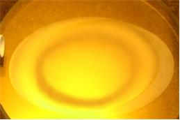
A picture of a real elliptical flat with elliptical fringes is adjacent. This has only one fringe visible which means it is about 0.5λ across the minor axis and also about 0.5λ across the major axis as well. There is a slight deviation from the pure elliptical shape of the fringe but the error is only about 1/10λ between the major and minor axis’s. This flat operating at 45 degrees in a Newtonian would theoretically be five times better than a 0.5λ conventional flat and its cheaper to produce! (It’s theoretical because the diffraction limited primary mirror is the real limit on performance.)
You may worry that the spherical surface produces spherical aberration? Please remember that if you had a telescope with a large focal ratio of say F/12 or F/15, it would hardly matter if the primary mirror was spherical or parabolic. At long focal ratios over say F/15, there is virtually no difference between spherical and parabolic curves and neither mirror would produce significant aberrations.
Now, – knowing that spherical aberrations are insignificant above say F/15, – compare that with a flat that might have a focal ratio between F/250 – F/2500! Spherical aberration will not affect performance.
The focal plane of the system will be moved by a small amount, – but you would have to be very clever to notice and measure it! A flat of 300,000” radius installed in a 20” F4 system will alter the focal length by about 0.01”
If you are still worried about having an elliptical flat behaving as a spherical secondary – remember that Cassegrain telescopes have secondary mirrors instead of an elliptical flat. They are curved many wavelengths away from flat, – but their images are not degraded.
If they did, – Not many people would be buying Schmidt Cassegrains from Celestron and Meade!
As our standard, Oldham Optical supply elliptical flats either better than one fringe (0.5λ), from flat, or a flat with elliptical fringes offering better performance. All flats supplied offer a performance matching a diffraction limited primary mirror.
Accurate Testing Of Optical Or Elliptical flats
While we use the technique of laying a flat under test on a known good flat and interpreting the resulting fringes as the main production test for our elliptical flats, – which is “straight-forward-Interferometry”, – we can test flats much more accurately if we need to.
If you have looked at other parts of our website, you will know we are not very enthusiastic about Interferometers. While a flat item is easier for an Interferometer to test because no extra optical components are needed to produce a spherical wave front, the fringes produced are still only 0.5λ apart. So expecting it to interpolate down to say 0.1λ is perhaps asking a lot of the equipment and set-up.
Its actually dead easy to test a flat surface “conventionally”. If we need to test a flat more accurately than with the production test then we can make use of a known good spherical mirror.
A spherical surface is always the easiest optical surface to produce. A knife edge test at the centre of curvature will easily detect problems in the spherical surface down well below 0.1λ.
Once we have a known good spherical mirror, the optical (or elliptical) flat is introduced into the test. Basically the optical flat is installed at 45 degrees to the optical path and the spherical mirror repositioned as shown in the adjacent diagram to reflect the rays back to the flat and then back to the knife edge.
This is a double pass Null test As it is double pass, a 0.1λ error appears to be 0.2λ. This test allows us to detect extremely small errors on the flat to below 0.1λ.
We could also use this for elliptical flats, but quite frankly its not economic to do so. We believe this web page has already demonstrated that an elliptical flat of extreme accuracy is not required in a conventional telescope.
OLDHAM OPTICAL